Foundations of Data Analytics

October 10, 2020

Contents:

1. Data Basics

---

Data Basics

• Data is formed of records.
  • These may also be called tuples, rows, samples etc.
• Each record has a number of attributes.
• Each attribute has a type.

Data Types

• Categoric or Nominal attributes take on one of a set of possible values.
  • E.g. Country, Marital Status.
  • They may not be able to be compared other than equal or not.
• Binary attributes take on one of two possible values.
• Ordered attributes take values from an ordered set.
• Numeric attributes measure quantities.
  • Can be integer, or real values.

Each attribute can be viewed as describing a random variable. Distributions from data are typically discrete.

Skewness

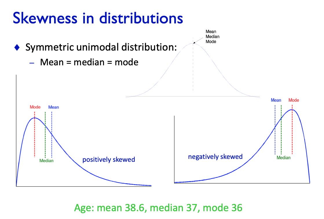
Distributions

See from slide 16 in data basics.

Q-Q Plots

Compare the quantile distribution to another.

• Allows comparison of attributes of different cardinality.
• If close to line $y=x$, this is evidence for same distribution.

Covariance

Calculated as:

$$Cov(X, Y) = E[(X - E[X]) (Y - E[Y])] \equiv E[XY] - E[X]E[Y]$$

If X and Y are independent, then covariance is 0. But, if covariance is 0, then X and Y can still be related.

PMCC

See from slide 26 in data basics.

Correlation for Ordered Data

• Can look at how the ranks of variables are correlated.

For correlation for categoric data, see from slide 31 in data basics.

Distance Functions

• Hamming Distance - Number of differences (e.g. number of differing binary digits).
• Euclidean Distance.
• Manhattan Distance - Absolute value distance.
• Minkowski Distances.

For Cosine Similarity, see slide 39.

Edit Distance

Counts the number of insertions, deletions, and changes of characters to turn one string into another.

Can be implemented using dynamic programming.

Data Preprocessing

• Data Cleaning - Remove noise, correct inconsistencies.
• Data Integration - Merge data from multiple sources.
• Data Reduction - Reduce data size for ease of processing.
• Data Transformation - Convert to different scales.

Missing Values

Approaches for handling:

• Drop the whole record.
• Fill in values manually.
• Accept and treat them as ‘unknown’.
• Fill in plausible values based on the data.
• Use rest of the data to infer the missing value.

Finding Outliers

For numeric data:

• Sanity check - are simple statistics different to expected?
• Visual - plot the data and look for spikes.
• Rule-based - set limits and declare an outlier if outside of bounds.
• Data-based - declare outlier if e.g. 6 standard deviations away from mean.

For categoric data:

• Can identify visually.
• Check for common typing mistakes etc.

To deal with outliers:

• Delete outliers - remove entire record.
• Clip outliers - change to maximum/minimum permitted value.
• Treat as missing value.

Random Sampling

A random sample is often enough when reducing a large dataset, but can miss out on small sub-populations.

Feature Selection

Includes principal component analysis, greedy attribute selection.

See from slide 55 in data basics.

---

Regression

Regression lets us predict a value for a numeric attribute.

• Based on principle of least squares.
  • This provides ‘best’ unbiased estimates for the parameters of the model.
  • Assumes unbiased independent noise with bounded variance.
• The mean minimises the squared deviation.
• The variance gives the minimal expected squared deviation.
• The standard deviation gives the root-mean-squared error.

Linear Model With Constant

• Fits a line of the form $y = ax + b$.
• $a = \frac{Cov(X, Y)}{Var(X)}$.
• $b = E[Y] - aE[X]$.
• Error or residual sum of squares is $n(Var(Y) - \frac{Cov^2(X, Y)}{Var(X)}$.

For Coefficient of Determination, see slide 13 in Regression.

Dealing with Categoric Attributes

• For simple binary attribute, create a variable which is 0 for one option and 1 for the other.
• For general categoric attributes, create a binary variable for each possibility.

For regularisation, see slide 30.

Correlations

Two perfectly correlated attributes can’t be used in regression. This would violate the requirement of no linearly dependent columns.

Predicting Categoric Values

See slides 36 onwards. Includes odds ratios, log odds ratios, logit transformation, logistic regression.

---

Classification

Classification is about creating models for categoric values.

The central concept is data = model + error.

• Attempt to extract a model from data.
• Error comes from noise, measurement error, random variation etc.
• We try to avoid modelling error - this leads to overfitting.
  • Can happen when a model has too many parameters.
  • Model ends up only describing the data and does not generalise.

Classification Process

1. Training - Obtain a data set with examples and a target attribute.
2. Evaluation - Apply the model to test data with hidden class value - evaluate quality of model by comparing prediction to hidden value.
3. Application - Apply model to new data with unknown class value, and monitor accuracy.

Evaluation Approaches

• Apply classifier to training data.
  • Risk of overfitting.
  • Some classifiers will achieve zero error.
• Hold back a subset of the training data for testing.
  • E.g. typically use 2/3 for training, 1/3 for testing.
  • Need to ensure balance - enough to train but also enough test.
• k-fold Cross-Validation.
  • Divide data into $k$ equal pieces (folds).
  • Use $k-1$ to form the training set.
  • Evaluate model accuracy on the remaining fold.
  • Repeat for each $k$ choices of training set.
• Stratified Cross-Validation.
  • Additionally, ensure each fold has the same class distribution.
  • Likely to hold if folds are chosen randomly.

Classifier Quality

• False Positive Rate - Fraction of negative values reported as positive.
  • FP / (FP + TN).
• True Positive Rate - Fraction of positive values reported as positive.
  • TP / (TP + FN).
• Precision - Fraction of positively reported values that are indeed positive.
  • TP / (TP + FP).
• Accuracy - (TP + TN) / (TP + TN + FN + FP).
• F1 Measure - Harmonic mean of precision and recall.
  • 2TP / (2TP + FP + FN).
• ROC and AUC - See slide 11.

Class Imbalance

• Accuracy is not always the best choice.
  • Class imbalance problem - what if one outcome is rare?
  • True positive rate may be better here.
• Some classifiers do not handle class imbalance well.
• Look at the confusion matrix - how each class is labeled.

Kappa Statistic

Compares accuracy to random guessing.

For computing kappa, see slide 13.

Kappa = 1 indicates perfect classification, kappa = 0 is random guessing.

Entropy

‘Informativeness’ is measured by entropy of the distribution.

• For a discrete PDF, entropy is $\sum_i p_i \log (1 / p_i)$.
• Measures the amount of ‘surprise’ in seeing each draw.
• Low entropy means low information/surprise.
• High entropy means more uncertainty of what is next.

Information Gain

General principle: pick the split that does most to separate classes, that is pick split with highest information gain.

The information gain from a proposed split is determined by the weighted sum of the entropy of the partitions.

For more information see slide 24.

• Algorithm is greedy, and does not guarantee the best tree, but usually works in practice.
• Prefers multi-valued splits, which may result in overfitting.

Decision Tree Algorithms

Different decision tree algorithms use different split rules. See slide 27 onwards.

Naive Bayes and SVM

See slide 35 onwards.

---

Clustering

Clustering aims to find classes without labelled examples. It is an ‘unsupervised’ learning method.

Distance Measurement

Some clustering algorithms assume a certain distance function.

We use distances that obey the metric rules:

• Identity - $d(x, y) = 0 \implies x = y$.
• Symmetry - $d(x, y) = d(y, x)$.
• Triangle Inequality - $d(x, z) \le d(x, y) + d(y, z)$.

Most distance measurements of interest are metrics.

Objective Functions

• K-Centre Objective - Minimise the diameter of each cluster, with $k$ centres.
• K-Medians Objective - Minimise the average distance from each point to its closest centre.
• K-Means Objective - Minimise the sum of squared distances between points and they closest centre.

It is NP-Hard to find an optimal clustering. There are two computational approaches:

• Approximation Algorithms - Guarantee some quality.
• Heuristic Methods - Give good results in practice but have limited or no guarantees.

Cluster Evaluation

• Harder to evaluate quality of a clustering.
• Can use a withheld class attribute to define a true clustering.
  • Can then study the confusion matrix comparing class to clusters.

Hierarchical Clustering

Hierarchical Agglomerative Clustering (HAC) creates binary tree structure of clusters.

Can use single-link, complete-link, or average-link.

Algorithm is polynomial.

TODO: Detail here.

Density-Based Clustering

• Seek clusters which are locally dense.
• Potentially allows finding complex cluster shapes.
• Possibly more robust to noise.

DBSCAN Algorithm from slide 48.

---

Recommendation

Recommender systems produce tailored recommendations.

Evaluation is similar to evaluating classifiers:

• Break labeled data into training and test data.
• For each test pair, predict the user score for the item.
• Measure the difference, and aim to minimise over N tests.

Neighbourhood Method

1. Find $k$ other users $K$ who are similar to target user $u$.
2. Combine the $k$ users’ weighted preferences.
3. Use these to make predictions for $u$.

Latent Factor Analysis

• Earlier we rejected methods based on features of items, since can not guarantee they will be available.
• Latent Factor Analysis tries to find ‘hidden’ features from the rating matrix.